Thursday, June 30, 2011
Libertarian summer camp
NPR's Planet Money podcast reports on the Porcupine Freedom Festival (PorcFest) held in Lancaster, NH.

Saturday, June 25, 2011
The impact of carbon taxes on New Hampshire manufacturing
Environmental economist Matthew Kahn estimates that a $15 per ton carbon tax would cause a 2.9% decline in New Hampshire manufacturing, or 1400 jobs.
The RGGI price is $1.89, suggesting a current, real-life decrease of approximately .4%, or 177 jobs.
Kahn adds:
The RGGI price is $1.89, suggesting a current, real-life decrease of approximately .4%, or 177 jobs.
Kahn adds:
Before opponents of cap and trade start to cite these numbers, it is important that clear headed folks keep in mind that this legislation will also stimulate the vaunted "green jobs" for the State. ...
The key point that nerds need to study is that such legislation simultaneously "destroys jobs" and "creates jobs". Here is another NBER study.
Sunday, June 19, 2011
Can New Hampshire afford to be last in economic growth?
In a recent Union Leader op-ed, Charlie Arlinghaus points out that New Hampshire, according to the latest BEA statistics, is last in economic growth in New England. Due to other data, he is "cautiously optimistic", but he argues that the low growth numbers should be interpreted as a warning sign by state policymakers.
Feeling warned, I took a closer look at the numbers. They do appear a little alarming, with New Hampshire in low-growth brown surrounded by states in high-growth blue (or at least middling white):

But what kind of warning is this?
Fortunately, the BEA provides detailed data on the contribution of different sectors to economic growth, so we can see exactly what's going on.
Browsing through their Excel file, it's clear that the housing sector is driving most of the difference. Here are the growth rates with housing excluded:
ME - 2.2%
CT - 2.9
NH - 2.9
RI - 2.9
VT - 3.0
MA - 3.6
To the extent that there is a warning, it's mostly about housing. Perhaps this is related to property taxes?
Of course, the difference could also be caused by factors unrelated to government policy, so we should interpret this data cautiously.
Feeling warned, I took a closer look at the numbers. They do appear a little alarming, with New Hampshire in low-growth brown surrounded by states in high-growth blue (or at least middling white):
But what kind of warning is this?
Fortunately, the BEA provides detailed data on the contribution of different sectors to economic growth, so we can see exactly what's going on.
Browsing through their Excel file, it's clear that the housing sector is driving most of the difference. Here are the growth rates with housing excluded:
ME - 2.2%
CT - 2.9
NH - 2.9
RI - 2.9
VT - 3.0
MA - 3.6
To the extent that there is a warning, it's mostly about housing. Perhaps this is related to property taxes?
Of course, the difference could also be caused by factors unrelated to government policy, so we should interpret this data cautiously.
Tuesday, June 14, 2011
The fallacy of composition, union version
Earlier, I used an equation and some data from Richard Freeman and James Medoff's book What Do Unions Do? to estimate the deadweight losses created by New Hampshire unions.
But I committed a subtle fallacy of composition, which biases my estimate downward. (The fallacy of composition arises when someone assumes that the part -- in this case, New Hampshire -- works the same as the whole -- the United States. It doesn't.)
I also want to clarify what exactly deadweight losses are, because, in retrospect, it seems that my earlier essay could easily be misinterpreted.
This is a diagram of the unionized labor market:

The demand curve slopes downward because, as the wage decreases, employers want to buy more labor. The supply curve slopes upward because, as the wage increases, more people want to work in this sector.
In a perfectly competitive market, the wages offered and the amount of labor hired would be set at the intersection of the supply and demand curves. If the wage were higher, the available workers would outnumber the available jobs, and employers would find that they could lower wages and still get all the labor they need. If the wage were lower, the available jobs would outnumber the available workers, and employers would have to raise wages in order to attract more workers into the market. This feedback effect leads employers to offer the wage where the two lines intersect, where the quantity of labor demanded and the quantity of labor supplied are equal.
But if workers bargain as a union, instead of accepting the competitive market wage, they can set the price-- in effect, choosing any point they'd like on the demand curve. Higher wages, however, come at the expense of fewer jobs, since employers want fewer workers at the higher wage.
This creates the deadweight loss. Some workers would like to work at the competitive market wage but cannot, and the businesses that would be happy to hire them at that wage are unable to. The potential benefits from employment that go unrealized are deadweight losses, and these losses are represented by the red triangle. The area of this triangle is what I was trying to find.
To arrive at the earlier conclusion, I used data from the federal level to estimate the elasticity of demand (a measure of the shape of the demand curve), but this is not similar to the elasticity of demand in the New Hampshire market by itself. The New Hampshire market in isolation has a higher elasticity of demand (that is, a flatter demand curve, meaning employers are more sensitive to changes in wages), because employers have the option of crossing the border into a different state. To do the same thing on the U.S. level would require leaving the country entirely, which is more difficult.
If the earlier graph represents my earlier estimate, the revised estimate should look more like this:

This graph shows that the union wage differential leads some businesses move to different states, so that the demand for New Hampshire union labor is lower. This increases deadweight loss, first because there are more people who would like to work at the market wage, but can't. Second, when businesses leave the state to avoid the higher union wages, the businesses do better, but the costs of moving are pure deadweight losses, as opposed to the higher wages, which redistribute wealth from employer to employee (businesses shift from blue to smaller red losses).
The takeaway from all of this is that my earlier estimate, that the deadweight losses due to unions were .05% of New Hampshire GDP, is probably too low. Watch out for that fallacy of composition.
But I committed a subtle fallacy of composition, which biases my estimate downward. (The fallacy of composition arises when someone assumes that the part -- in this case, New Hampshire -- works the same as the whole -- the United States. It doesn't.)
I also want to clarify what exactly deadweight losses are, because, in retrospect, it seems that my earlier essay could easily be misinterpreted.
This is a diagram of the unionized labor market:

The demand curve slopes downward because, as the wage decreases, employers want to buy more labor. The supply curve slopes upward because, as the wage increases, more people want to work in this sector.
In a perfectly competitive market, the wages offered and the amount of labor hired would be set at the intersection of the supply and demand curves. If the wage were higher, the available workers would outnumber the available jobs, and employers would find that they could lower wages and still get all the labor they need. If the wage were lower, the available jobs would outnumber the available workers, and employers would have to raise wages in order to attract more workers into the market. This feedback effect leads employers to offer the wage where the two lines intersect, where the quantity of labor demanded and the quantity of labor supplied are equal.
But if workers bargain as a union, instead of accepting the competitive market wage, they can set the price-- in effect, choosing any point they'd like on the demand curve. Higher wages, however, come at the expense of fewer jobs, since employers want fewer workers at the higher wage.
This creates the deadweight loss. Some workers would like to work at the competitive market wage but cannot, and the businesses that would be happy to hire them at that wage are unable to. The potential benefits from employment that go unrealized are deadweight losses, and these losses are represented by the red triangle. The area of this triangle is what I was trying to find.
To arrive at the earlier conclusion, I used data from the federal level to estimate the elasticity of demand (a measure of the shape of the demand curve), but this is not similar to the elasticity of demand in the New Hampshire market by itself. The New Hampshire market in isolation has a higher elasticity of demand (that is, a flatter demand curve, meaning employers are more sensitive to changes in wages), because employers have the option of crossing the border into a different state. To do the same thing on the U.S. level would require leaving the country entirely, which is more difficult.
If the earlier graph represents my earlier estimate, the revised estimate should look more like this:

This graph shows that the union wage differential leads some businesses move to different states, so that the demand for New Hampshire union labor is lower. This increases deadweight loss, first because there are more people who would like to work at the market wage, but can't. Second, when businesses leave the state to avoid the higher union wages, the businesses do better, but the costs of moving are pure deadweight losses, as opposed to the higher wages, which redistribute wealth from employer to employee (businesses shift from blue to smaller red losses).
The takeaway from all of this is that my earlier estimate, that the deadweight losses due to unions were .05% of New Hampshire GDP, is probably too low. Watch out for that fallacy of composition.
Thursday, May 26, 2011
Why are state legislators so crazy lately?
Betsy Russell at the Idahoan Spokesman-Review offers some informed speculation, drawing on a few high-profile political scientists.
HT: Seth Masket.
HT: Seth Masket.
Wednesday, May 25, 2011
Apples, oranges, and right-to-work
Don Ewing at GraniteGrok argues that right-to-work laws decrease unemployment, increase personal income growth, and increase private sector employment.
But Don forgets that correlation does not imply causation.
In real life, states with right-to-work laws differ systematically from states without them, and this invalidates the comparisons.
Wikipedia has a convenient map of right-to-work states (in blue):
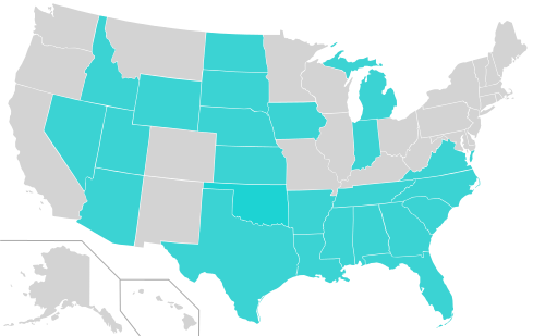
Clearly these states are not randomly distributed across the map, leaving plenty of room for geographical factors to influence the numbers (notably unemployment rates).
The personal income measure used by the BEA— I think this is what Ewing was referencing— is the sum of all income earned, meaning that immigration patterns influence the growth rates. (A growing population leads to a higher total personal income.) And, according to research by Harvard economist Edward Glaeser, among others, one of the main determinants of immigration is the elasticity of the housing supply— that is, how easy it is to build new houses as the price of houses increases. For all we know, personal income growth in right-to-work states is being driven by the housing market. The same applies to growth in private sector employment.
Or the differences could be driven by one of a thousand other factors.
From what I've seen, using statistics to tease out the effects of particular state policies is ridiculously hard to do, and requires a much stronger statistical background than I have. This is a lot of the reason why I didn't even broach the subject in my union essay.
A quick search for an academic analysis of the issue found only this paper by Thomas Holmes. By comparing bordering counties in different states, he finds that a business-friendly regulatory climate increases the share of employment in manufacturing by about one third. But this study looks only at manufacturing, and only at counties on the borders of states (which means the estimate is inflated by an unknown amount). And the contribution of right-to-work laws to business-friendly regulatory climates is unknown.
So we can guess that right-to-work laws will increase the share of our employment in manufacturing by anywhere from zero to one-third. Which doesn't get us very far.
But Don forgets that correlation does not imply causation.
In real life, states with right-to-work laws differ systematically from states without them, and this invalidates the comparisons.
Wikipedia has a convenient map of right-to-work states (in blue):
Clearly these states are not randomly distributed across the map, leaving plenty of room for geographical factors to influence the numbers (notably unemployment rates).
The personal income measure used by the BEA— I think this is what Ewing was referencing— is the sum of all income earned, meaning that immigration patterns influence the growth rates. (A growing population leads to a higher total personal income.) And, according to research by Harvard economist Edward Glaeser, among others, one of the main determinants of immigration is the elasticity of the housing supply— that is, how easy it is to build new houses as the price of houses increases. For all we know, personal income growth in right-to-work states is being driven by the housing market. The same applies to growth in private sector employment.
Or the differences could be driven by one of a thousand other factors.
From what I've seen, using statistics to tease out the effects of particular state policies is ridiculously hard to do, and requires a much stronger statistical background than I have. This is a lot of the reason why I didn't even broach the subject in my union essay.
A quick search for an academic analysis of the issue found only this paper by Thomas Holmes. By comparing bordering counties in different states, he finds that a business-friendly regulatory climate increases the share of employment in manufacturing by about one third. But this study looks only at manufacturing, and only at counties on the borders of states (which means the estimate is inflated by an unknown amount). And the contribution of right-to-work laws to business-friendly regulatory climates is unknown.
So we can guess that right-to-work laws will increase the share of our employment in manufacturing by anywhere from zero to one-third. Which doesn't get us very far.
Monday, May 23, 2011
Our modest recession
Changes in unemployment from 2007 to 2010, by state:

According to Paul Krugman, New Hampshire fared well, at least in part, because it's a "cold [place] where nobody lives".
... Guess we can't have it all.
According to Paul Krugman, New Hampshire fared well, at least in part, because it's a "cold [place] where nobody lives".
... Guess we can't have it all.
Subscribe to:
Posts (Atom)